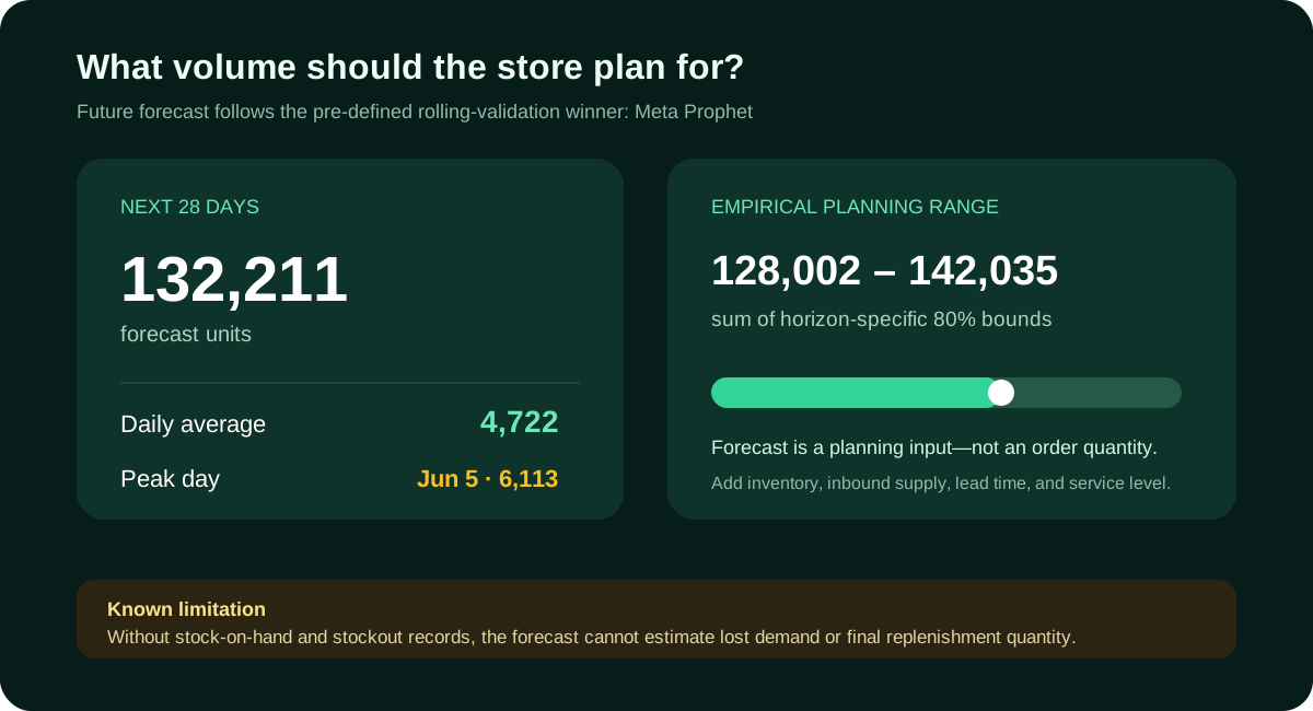
Retail Demand Forecasting: Which Model Generalizes Best?

3,049
Items in scope
5.89%
Rolling WAPE
5.75%
Final-test WAPE
Tech Stack
Description
This project demonstrates the time-series forecasting and systematic cross-validation work highlighted in my resume through a reproducible retail demand-planning workflow.
The central comparison spans simple seasonal baselines, classical statistical models, feature-driven machine learning, Meta Prophet, and Google TimesFM 3.0. Every model uses the same rolling forecast origins, 28-day horizon, and error definitions.
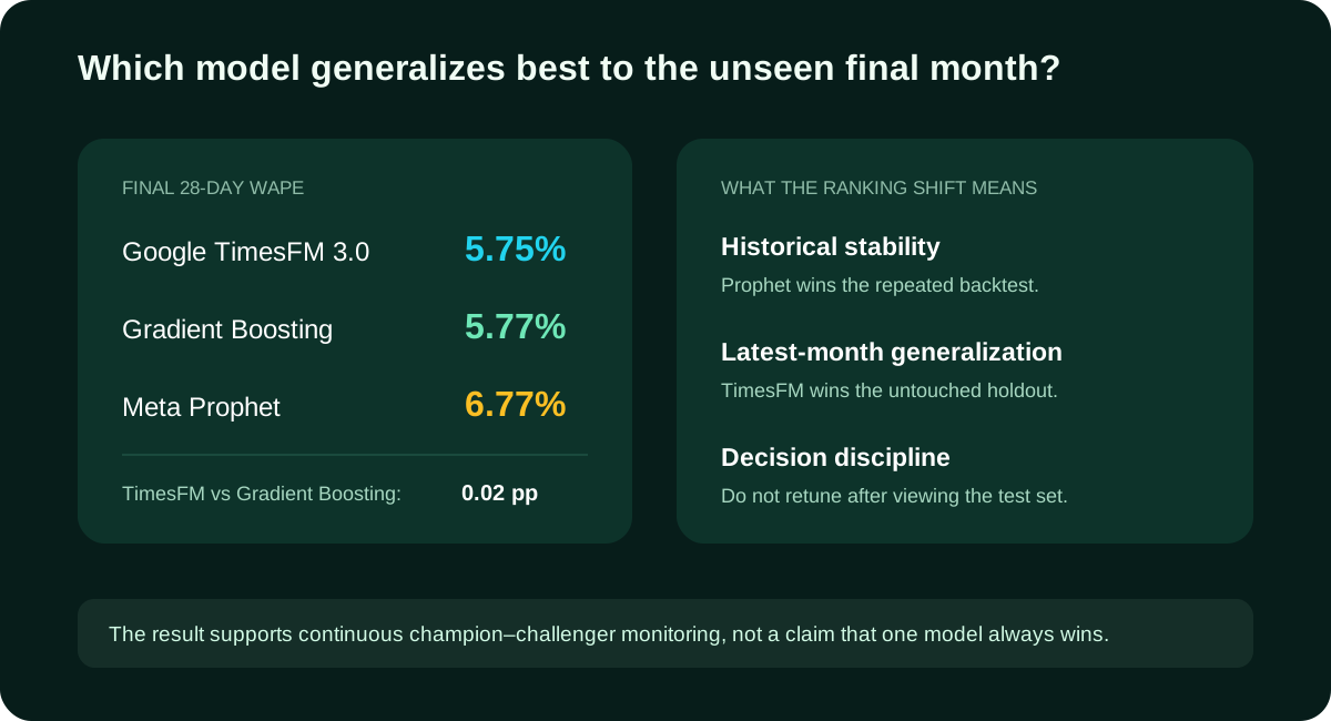
The project separates model selection from final testing. Prophet is the historical rolling-validation champion, while zero-shot TimesFM performs best on the newest untouched month. The difference becomes a monitoring decision rather than a misleading winner-takes-all claim.
- Built a continuous 1,941-day store series across 3,049 items with calendar and price signals.
- Engineered leakage-safe lags and rolling features for a direct 28-day machine-learning forecast.
- Compared seven models across four rolling windows with MAE, RMSE, WAPE, and signed bias.
- Benchmarked Google TimesFM 3.0 zero-shot against Meta Prophet, Gradient Boosting, and statistical baselines.
- Translated the selected forecast into a 132,211-unit planning baseline with explicit uncertainty and inventory limitations.
Project Highlights
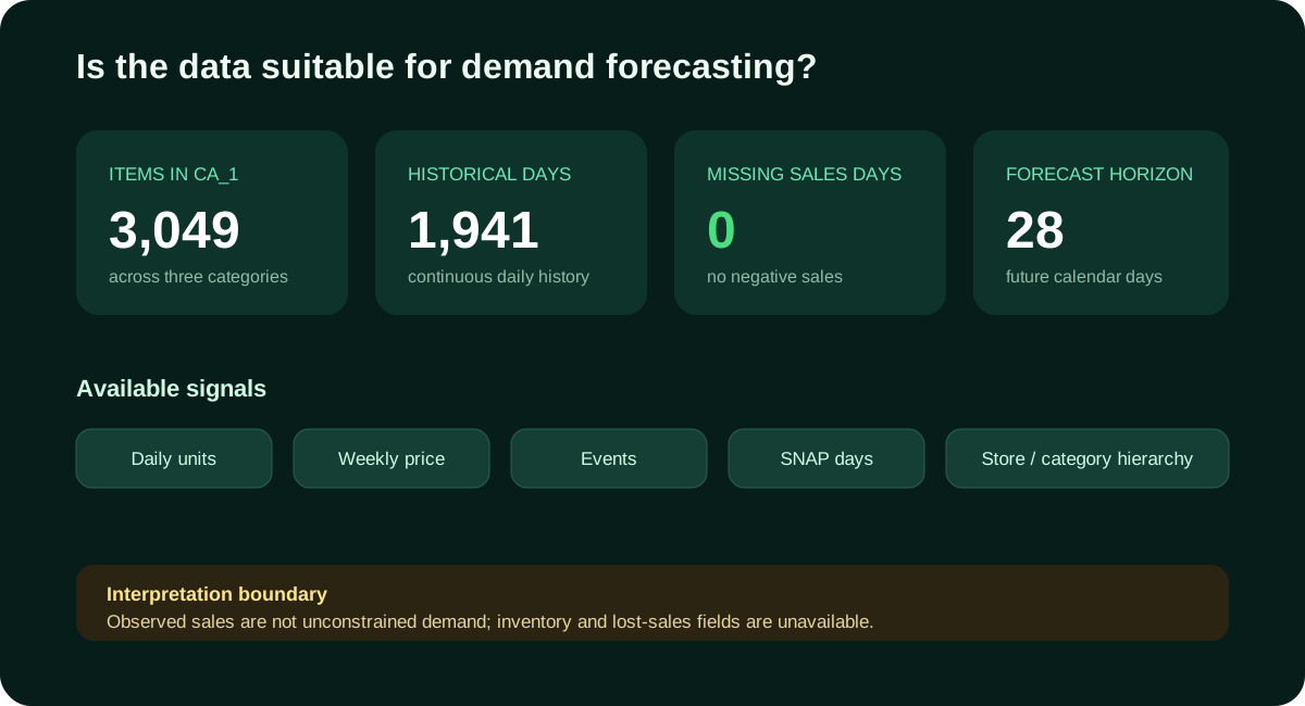
Q1. Is the data suitable for demand forecasting?
Question: Can the source tables support a reliable store-level 28-day forecast? Analysis: I reconciled daily unit sales, weekly prices, calendar events, benefit-program dates, and the store-category hierarchy. The selected store contains 3,049 items across three categories and 1,941 continuous historical days. Finding: The series has no missing sales dates or negative values, and it shows both changing sales levels and strong weekly seasonality. The target is observed store sales—not unconstrained demand—because inventory-on-hand and lost-sales fields are unavailable.
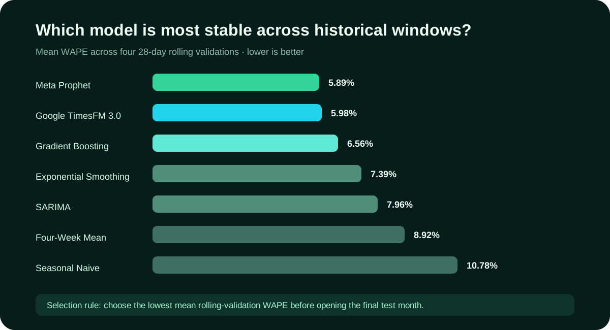
Q2. Which model is most stable across historical windows?
Question: Which method performs most reliably when the forecast origin moves through time? Analysis: Seven models face the same four rolling 28-day validation windows: two seasonal baselines, Exponential Smoothing, SARIMA, Gradient Boosting, Meta Prophet, and Google TimesFM 3.0. Selection is based on mean WAPE before viewing the final test month. Finding: Meta Prophet ranks first at 5.89% mean WAPE, closely followed by zero-shot TimesFM at 5.98% and Gradient Boosting at 6.56%. Prophet is selected as the historical champion under the pre-defined rule.
Q3. Which model generalizes best to the unseen final month?
Question: Does the rolling-validation winner remain best on a completely untouched 28-day period? Analysis: After model selection, I evaluate every candidate once on the reserved final month using MAE, RMSE, WAPE, and signed bias. Finding: Google TimesFM 3.0 ranks first at 5.75% WAPE, almost tied with Gradient Boosting at 5.77%; Prophet records 6.77%. The ranking shift supports champion–challenger monitoring rather than a claim that one model always wins. TimesFM is presented only as a non-commercial research benchmark under its current weight license.
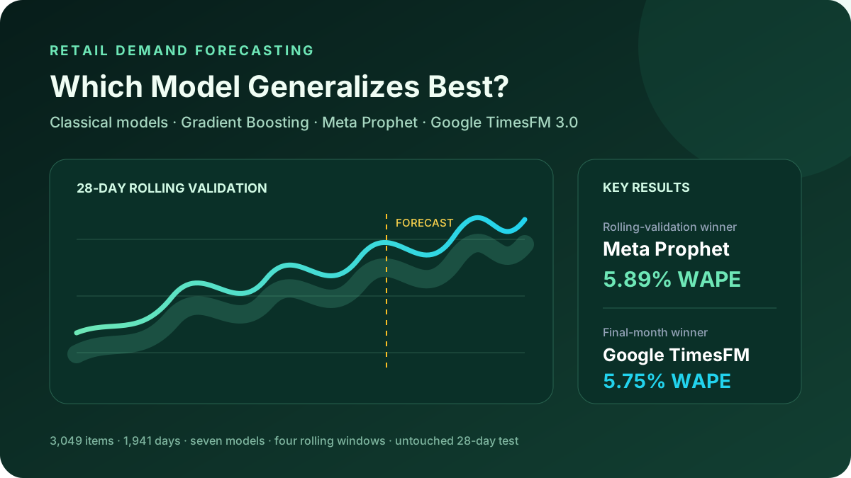
Q4. What volume should the store plan for?
Question: How should the selected forecast be translated into a usable 28-day planning range? Analysis: Following the pre-defined rolling-validation decision, Prophet is refit on all 1,941 historical days. Horizon-specific errors from the four backtests form an empirical 80% interval. Finding: The forecast is 132,211 units over 28 days, averaging 4,722 per day, with summed daily bounds of 128,002 to 142,035 units. This is a capacity and purchasing-budget input—not a final order quantity—until inventory, inbound supply, lead time, and service level are added.